KV Caching in LLMs: A Guide for Developers

In this article, you will learn how key-value (KV) caching eliminates redundant computation in autoregressive transformer inference to dramatically improve generation speed.

Topics we will cover include:

Why autoregressive generation has quadratic computational complexity How the attention mechanism produces query, key, and value representations How KV caching works in practice, including pseudocode and memory trade-offs

Let’s get started.

KV Caching in LLMs: A Guide for Developers
Image by Editor

Introduction

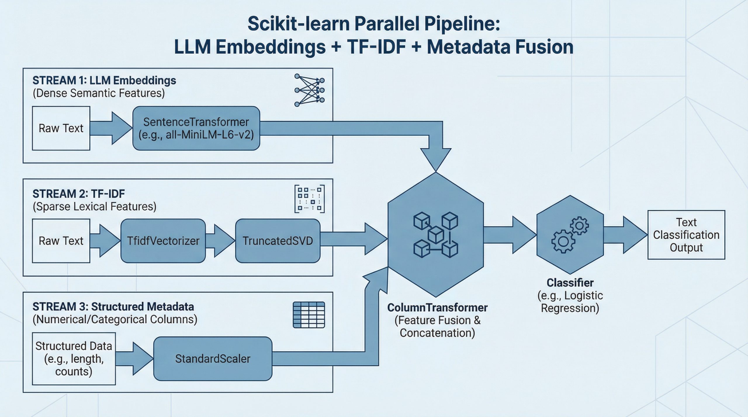
Language models generate text one token at a time, reprocessing the entire sequence at each step. To generate token n, the model recomputes attention over all (n-1) previous tokens. This creates \( O(n^2) \) complexity, where computation grows quadratically with sequence length, which becomes a major bottleneck for inference speed.

Key-value (KV) caching eliminates this redundancy by leveraging the fact that the key and value projections in attention do not change once computed for a token. Instead of recomputing them at each step, we cache and reuse them. In practice, this can reduce redundant computation and provide 3–5× faster inference, depending on model size and hardware.

Prerequisites

This article assumes you are familiar with the following concepts:

Neural networks and backpropagation The transformer architecture The self-attention mechanism in transformers Matrix multiplication concepts such as dot products, transposes, and basic linear algebra

If any of these feel unfamiliar, the resources below are good starting points before reading on. The Illustrated Transformer by Jay Alammar is one of the clearest visual introductions to transformers and attention available. Andrej Karpathy’s Let’s Build GPT walks through building a transformer from scratch in code.

Both will give you a solid foundation to get the most out of this article. That said, this article is written to be as self-contained as possible, and many concepts will become clearer in context as you go.

The Computational Problem in Autoregressive Generation

Large language models use autoregressive generation — producing one token at a time — where each token depends on all previous tokens.

Let’s use a simple example. Start with the input word: “Python”. Suppose the model generates:

Input: "Python" Step 1: "is" Step 2: "a" Step 3: "programming" Step 4: "language" Step 5: "used" Step 6: "for" ...

Input: "Python"

Step 1: "is"

Step 2: "a"

Step 3: "programming"

Step 4: "language"

Step 5: "used"

Step 6: "for"

...

Here is the computational problem: to generate “programming” (token 3), the model processes “Python is a”. To generate “language” (token 4), it processes “Python is a programming”. Every new token requires reprocessing all previous tokens.

Here is a breakdown of tokens that get reprocessed repeatedly:

“Python” gets processed 6 times (once for each subsequent token) “is” gets processed 5 times “a” gets processed 4 times “programming” gets processed 3 times

The token “Python” never changes, yet we recompute its internal representations over and over. In general, the process looks like this:

Generate token 1: Process 1 position Generate token 2: Process 2 positions Generate token 3: Process 3 positions ... Generate token n: Process n positions

Generate token 1: Process 1 position

Generate token 2: Process 2 positions

Generate token 3: Process 3 positions

...

Generate token n: Process n positions

This gives us the following complexity for generating n tokens:
\[
\text = 1 + 2 + 3 + \cdots + n = \frac \approx O(n^2)
\]

Understanding the Attention Mechanism and KV Caching

Think of attention as the model deciding which words to focus on. The self-attention mechanism at the core of transformers computes:

\[
\text(Q, K, V) = \text\left(\frac}\right)V
\]

The mechanism creates three representations for each token:

Query (Q): Each token uses its query to search the sequence for relevant context needed to be interpreted correctly. Key (K): Each token broadcasts its key so other queries can decide how relevant it is to what they are looking for. Value (V): Once a query matches a key, the value is what actually gets retrieved and used in the output.

Each token enters the attention layer as a \( d_} \)-dimensional vector. The projection matrices \( W_Q \), \( W_K \), and \( W_V \) — learned during training through backpropagation — map it to \( d_k \) per head, where \( d_k = d_} / \text \).

During training, the full sequence is processed at once, so Q, K, and V all have shape [seq_len, d_k], and \( QK^T \) produces a full [seq_len, seq_len] matrix with every token attending to every other token simultaneously.

At inference, something more interesting happens. When generating token \( t \), only Q changes. The K and V for all previous tokens \( 1 \ldots t-1 \) are identical to what they were in the previous step. Therefore, it is possible to cache these key (K) and value (V) matrices and reuse them in subsequent steps. Hence the name KV caching.

Q has shape [1, d_k] since only the current token is passed in, while K and V have shape [seq_len, d_k] and [seq_len, d_v], respectively, growing by one row each step as the new token’s K and V are appended.

With these shapes in mind, here is what the formula computes:

\( QK^T \) computes a dot product between the current token’s query and every cached key, producing a [1, seq_len] similarity score across the full history. \( 1/\sqrt \) scales scores down to prevent dot products from growing too large and saturating the softmax. \( \text(\cdot) \) converts the scaled scores into a probability distribution that sums to 1. Multiplying by V weights the value vectors by those probabilities to produce the final output. Comparing Token Generation With and Without KV Caching

Let’s trace through our example with concrete numbers. We will use \( d_} = 4 \). Real models, however, typically use 768–4096 dimensions.

Input: “Python” (1 token). Suppose the language model generates: “is a programming language”.

Without KV Caching

At each step, K and V are recomputed for every token in the sequence, and the cost grows as each token is added.

Step Sequence K & V Computed 0 Python Python 1 Python is Python, is 2 Python is a Python, is, a 3 Python is a programming Python, is, a, programming 4 Python is a programming language Python, is, a, programming, language With KV Caching

With KV caching, only the new token’s K and V are computed. Everything prior is retrieved directly from the cache.

Step Sequence K & V Computed & Cached K & V Retrieved 0 Python Python — 1 Python is is Python 2 Python is a a Python, is 3 Python is a programming programming Python, is, a 4 Python is a programming language language Python, is, a, programming Implementing KV Caching: A Pseudocode Walkthrough Initializing the Cache

The attention layer holds the cache as part of its state. There are two slots for keys and values that start empty and fill during generation.

class MultiHeadAttentionWithCache: def __init__(self, d_model, num_heads): self.d_model = d_model self.num_heads = num_heads self.d_k = d_model // num_heads # Learned projection matrices self.W_Q = Linear(d_model, d_model) self.W_K = Linear(d_model, d_model) self.W_V = Linear(d_model, d_model) self.W_O = Linear(d_model, d_model) # Cache storage (initially None) self.cache_K = None self.cache_V = None

class MultiHeadAttentionWithCache:

    def __init__(self, d_model, num_heads):

        self.d_model = d_model

        self.num_heads = num_heads

        self.d_k = d_model // num_heads

 

        # Learned projection matrices

        self.W_Q = Linear(d_model, d_model)

        self.W_K = Linear(d_model, d_model)

        self.W_V = Linear(d_model, d_model)

        self.W_O = Linear(d_model, d_model)

 

        # Cache storage (initially None)

        self.cache_K = None

        self.cache_V = None

Only K and V are cached. Q is always computed because it represents the current query. Each layer in the model maintains its own independent cache.

Using Caching Logic in the Forward Pass

Before any caching logic runs, the input is projected into Q, K, and V and reshaped across attention heads.

def forward(self, x, use_cache=False): batch_size, seq_len, _ = x.shape Q = self.W_Q(x) K_new = self.W_K(x) V_new = self.W_V(x) # [batch, seq_len, d_model] -> [batch, num_heads, seq_len, d_k] Q = reshape_to_heads(Q, self.num_heads) K_new = reshape_to_heads(K_new, self.num_heads) V_new = reshape_to_heads(V_new, self.num_heads)

def forward(self, x, use_cache=False):

    batch_size, seq_len, _ = x.shape

 

    Q = self.W_Q(x)

    K_new = self.W_K(x)

    V_new = self.W_V(x)

 

    # [batch, seq_len, d_model] -> [batch, num_heads, seq_len, d_k]

    Q = reshape_to_heads(Q, self.num_heads)

    K_new = reshape_to_heads(K_new, self.num_heads)

    V_new = reshape_to_heads(V_new, self.num_heads)

K_new and V_new represent only the current input. They have not been appended to the cache yet. The reshape operation splits d_model evenly across heads so each head attends to a different subspace.

Updating the KV Cache

This is the key step. On the first call, the cache is seeded, and on every subsequent call, new keys and values are appended to it.

if use_cache: if self.cache_K is None: self.cache_K = K_new self.cache_V = V_new else: self.cache_K = concat([self.cache_K, K_new], dim=2) self.cache_V = concat([self.cache_V, V_new], dim=2) K = self.cache_K V = self.cache_V else: K = K_new V = V_new

if use_cache:

    if self.cache_K is None:

        self.cache_K = K_new

        self.cache_V = V_new

    else:

        self.cache_K = concat([self.cache_K, K_new], dim=2)

        self.cache_V = concat([self.cache_V, V_new], dim=2)

 

    K = self.cache_K

    V = self.cache_V

else:

    K = K_new

    V = V_new

Concatenation happens along dim=2, the sequence dimension, so the cache grows one token at a time. When caching is active, K and V always contain the full history — meaning every token the model has seen in this session.

Computing Attention

With K and V now containing the full history, attention runs as usual. The only difference is that seq_len_k is longer than seq_len_q during decoding.

scores = matmul(Q, transpose(K)) / sqrt(self.d_k) # scores: [batch, num_heads, seq_len_q, seq_len_k] mask = create_causal_mask(Q.shape[2], K.shape[2]) scores = masked_fill(scores, mask == 0, -inf) attn_weights = softmax(scores, dim=-1) output = matmul(attn_weights, V) output = reshape_from_heads(output) output = self.W_O(output) return output

scores = matmul(Q, transpose(K)) / sqrt(self.d_k)

# scores: [batch, num_heads, seq_len_q, seq_len_k]

 

mask = create_causal_mask(Q.shape[2], K.shape[2])

scores = masked_fill(scores, mask == 0, -inf)

 

attn_weights = softmax(scores, dim=-1)

output = matmul(attn_weights, V)

 

output = reshape_from_heads(output)

output = self.W_O(output)

 

return output

The causal mask ensures position \( i \) can only attend to positions \( \leq i \), preserving autoregressive order. The final projection through W_O recombines all heads back into a single \( d_} \)-dimensional output.

Managing the Cache

Between generation requests, the cache must be cleared because stale keys and values from a previous session can corrupt the next.

def reset_cache(self): self.cache_K = None self.cache_V = None

def reset_cache(self):

    self.cache_K = None

    self.cache_V = None

This should always be called before starting a new generation. Forgetting this is a common source of subtle, hard-to-debug issues where outputs appear contextually contaminated.

Generating Text

The generation process has two distinct phases: a parallel prefill over the entire prompt, followed by a sequential decode loop that adds one token at a time.

def generate_with_kv_cache(model, input_ids, max_new_tokens): model.reset_all_caches() # Prefill: process full prompt in parallel, populates cache logits = model(input_ids, use_cache=True) for _ in range(max_new_tokens): next_token_logits = logits[:, -1, :] next_token = argmax(next_token_logits, keepdim=True) input_ids = concat([input_ids, next_token], dim=1) # Only the new token is passed — cache handles the rest logits = model(next_token, use_cache=True) return input_ids

def generate_with_kv_cache(model, input_ids, max_new_tokens):

    model.reset_all_caches()

 

    # Prefill: process full prompt in parallel, populates cache

    logits = model(input_ids, use_cache=True)

 

    for _ in range(max_new_tokens):

        next_token_logits = logits[:, -1, :]

        next_token = argmax(next_token_logits, keepdim=True)

        input_ids = concat([input_ids, next_token], dim=1)

 

        # Only the new token is passed — cache handles the rest

        logits = model(next_token, use_cache=True)

 

    return input_ids

During prefill, the full prompt is processed in one forward pass, which fills the cache with K and V for every input token. During decoding, each step passes only a single new token. The model attends to all prior context through the cache, not by reprocessing it. This is why generation scales efficiently: compute per step remains constant regardless of how long the sequence becomes.

To summarize why this works:

Token 1: The model sees [input], and the cache stores K and V for the input Token 2: The model sees [token1], but attention uses cached K and V from the input as well Token 3: The model sees [token2], but attention uses K and V from input, token1, and token2

As you can see, memory grows linearly with sequence length, which can become prohibitive for very long contexts.

Wrapping Up

KV caching addresses a fundamental limitation in autoregressive text generation, where models repeatedly recompute attention projections for previously processed tokens. By caching the key and value matrices from the attention mechanism and reusing them across generation steps, we eliminate redundant computation that would otherwise grow quadratically with sequence length.

This significantly speeds up large language model inference. The trade-off is increased memory usage, as the cache grows linearly with sequence length. In most real-world systems, this memory cost is justified by the substantial improvements in inference latency.

Understanding KV caching provides a foundation for more advanced inference optimizations. From here, you can explore techniques such as quantized caches, sliding-window attention, and speculative decoding to push performance even further.

References & Further Reading

View Original Article