Excel's best cleanup trick is hidden behind Ctrl+G

Most people I know hit Ctrl+C and Ctrl+V in Excel hundreds of times a day, but have never pressed Ctrl+G. They're missing out because the Go To dialog that opens is just the front door, and the real cleanup power lives behind a small button labeled Special.

It can grab every blank cell, every formula, every error, and every visible row in your selection in one click. I lean on it more than any other everyday Excel keyboard shortcut I'd hate to lose, and once you see what it does to a messy sheet, you'll have a hard time going back.

Related Ctrl+G opens way more than a basic Go To dialog

Press Ctrl+G, and the window that pops up looks ordinary — a text box, an OK button, and a Special button tucked in the bottom-left corner. That Special button is the whole reason the keystroke earns its place in my workflow.

Click it, and you get a menu most people have never opened: blanks, constants, formulas, conditional formats, data validation, objects, visible cells only, and row differences, among others. Each option tells Excel to select every cell in your active range that matches that condition.

You can reach the same menu through Find & Select on the Home tab, but that's three clicks deep. Ctrl+G then Special is two keystrokes and one click. Over the course of a workday spent cleaning sales data and chasing down stray entries, that adds up.

Deleting blank rows is the easiest cleanup win Screenshot by Yasir Mahmood

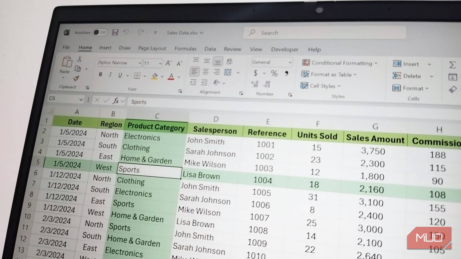
My sales data has 33 rows of actual entries and a long tail of blank rows underneath, leftover space that someone never trimmed before sending the file over. Sorting doesn't help as empty rows already collect at the bottom. Manually deleting them works on a small sheet, but it's a different story when you're facing a few thousand rows. Here's the cleaner way:

Select the column you want to scan for blanks. The Salesperson column works as a good anchor in my case. Press Ctrl + G, then click Special. Choose Blanks and click OK. Right-click any highlighted cell and pick Delete > Entire row.

Excel removes every row that has a missing value in that column without disturbing the rest of the structure. On the sales sheet, this trims the dead space in about five seconds. On a 6,000-row sheet, it still takes about five seconds.

Auditing formulas takes seconds when you select them all at once Color-coding your calculations makes errors easier to spot Screenshot by Yasir Mahmood

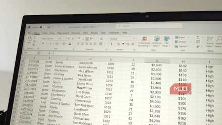
In a busy sheet, hardcoded numbers and formulas look identical until something breaks. The Commission and Profit Margin columns in my sales workbook run on LET formulas, but if I overwrite one cell with a static number by mistake, nothing visually changes — until next month's totals come in wrong.

However, Ctrl + G > Special > Formulas highlights every formula cell in your selection at once. From there, I apply a fill color to them so calculations stand out from inputs, which is one of the formatting tricks I use to make calculated cells more visible.

The dialog also lets you further narrow it down to Numbers, Text, Logicals, or Errors. If you only want the formula errors, that last filter takes you straight to the broken cells without writing IFERROR around every calculation.

Visible cells only is the option that power users swear by Screenshot by Yasir Mahmood

When I've manually hidden rows in a sales report — collapsing the South and East regions to focus on North and West — the obvious move is to copy what's left and paste it elsewhere. Excel doesn't always cooperate. Hidden rows tend to ride along with the visible ones, especially when you're working with grouped or outlined data. Here's the fix:

Hide or collapse the rows you don't want. Select the visible range. Press Ctrl + G, then click Special. Pick Visible cells only and click OK. Copy and paste, and now only the visible rows transfer.

This is also the clean way to copy from a grouped outline without having to ungroup first. Any time you've narrowed a dataset for someone else, this is the keystroke that keeps the paste honest.

Screenshot by Yasir Mahmood

The headline cleanup wins are blanks, formulas, and visible cells, but the rest of the Go To Special menu is worth knowing, too. Notes jump to every annotated cell at once, which helps when you're stripping markup before sharing a workbook with a client.

Objects selects every image, chart, and shape in your sheet, which beats clicking through them individually when you want to delete or move a batch. Constants does the inverse of the Formulas option — it isolates every hardcoded value so you can audit your inputs without touching the calculations. That makes it a good companion to data validation rules that block bad entries before they hit your sheet.

Row Differences is the quiet star here. Pick a row, run it, and Excel highlights the one cell that doesn't match the pattern of its neighbors. That's a quick consistency check without writing a helper formula.

Where I'm taking Ctrl+G next Pairing it with conditional formatting is the obvious follow-up

The next thing I want to layer on top of this is conditional formatting that flags formula cells the moment they're written, so the audit pass becomes visual instead of manual. There's a balance to strike, though — too many overlapping rules and the sheet starts looking like a stained-glass window, which is why keeping conditional formatting under control matters as much as setting it up.

The deeper I get into Excel, the more the useful features turn out to live one click past where most people stop looking. Ctrl+G is the prototype for that pattern, and there's more of the menu left to explore.

View Original Article